Tutorial on Linearized MPC controller

This is a tutorial on the implementation of successive linearization based model predictive control in Matlab. This script shows how to implement the controller for a nonlinear system described by the differential equation

\begin{align} \dot{x} &= f(x,u) \newline y&=Cx+Du \end{align}

For details of derivation and background information, please refer to Zhakatayey et al. “Successive linearization based model predictive control of variable stiffness actuated robots.”.

Problem statement

MPC controller requires several parameters:

np - horizon length (number of time steps in the prediction horizon)

Q - a weight matrix representing relative importance of states (also we use vector ‘wx’)

R - a weight matrix penalizing large values of control inputs ( vector ‘wu’)

The general Model Predictive Control (MPC) can be formulated as an optimization problem with horizon length \(np\):

subject to:

In order to solve this problem, we can use the built-in quadratic programmer quadprog() in Matlab. Please refer to the documentation of quadprog() function for details. In fact, any nonlinear optimization problem solver can be used to solve this problem. For example, qpOASES is suitable for real-time operation of control systems thanks to its ability to find solutions quickly.

Block Diagram of the Successive Linearization Model Predictive Controller

Tutorial objectives

This tutorial covers basic implementation of the SLMPC controller. This consists of:

1. Linearization of model
2. Discretization of linearized model
3. Solving SL-MPC optimization problem with simple constraints

In this tutorial, we use a simple pendulum for the test case with the equation of motion:

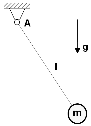
Following MATLAB code shows our implementation:

close all; clear; clc;
% global parameters associated with dynamic model of the system 
sys.g = 9.81;
sys.l = 0.1;
sys.b = 0.2;
% this is matrices to represent output as y=C*x+D*u
C = eye(2);  
D = [0;0];
%initial point of states
x = [0.001; 0];
%control input max and min values
ui=0;
umax = 80;
umin =-20;
% IMPORTANT PARAMETERS
np = 40;       % horizon length 
nx = 2;        % number of states 
nu = 1;        % number of inputs
no = size(C,1);% number of outputs
Ts = 0.001;    % step size
Tfinal = 0.5;  % final time
wx = [1000 1]; % relative importance of states
wu = 0.00001;  % penalizing weights of control inputs
% generating simple step reference of the form [0.5 ; 0] 
ref =0.5*[ones(1,Tfinal/Ts +np);zeros(1,Tfinal/Ts +np)];
% model is anonymous function that represents the equation which describes 
% system dynamic model and in the form of dx/dt =f(x,u). 
model = @(x,u) nonlin_eq(x,u,sys); 
% FOR MPC CONTROLLER
rr = zeros(np*nx,1);
y  = zeros(no,Tfinal/Ts);
uh = zeros(nu,Tfinal/Ts);
%constraints for inputs in the whole horizon in the form of Acon*u <=Bcon
[Acon,Bcon] = simple_constraints(umax,umin,np,nu);
% weighting coefficient reflecting the relative importance of states and control inputs 
Q = diag(repmat(wx, 1, np)); 
R = diag(repmat(wu, 1, np));
% Setting the quadprog with 200 iterations at maximum
opts = optimoptions('quadprog', 'MaxIter', 200, 'Display','off');
% MAIN SIMULATION LOOP
for t=1:Tfinal/Ts
    
    rr =  ref_for_hor(rr,ref,t,np,nx);% reference vector for whole horizon  
    y(:,t) = C*x+D*ui;                % evaluating system output 
    [x, dx] = RK4(x,ui,Ts,model);     % i.e. simulate one step forward with Runge-Kutta 4 order integrator
    [A, B, K] = linearize_model(x,dx,ui,sys);                           % linearization step
    [Ad,Bd,Kd] = discretize(A,B,K,Ts);                              % discretization step
    [G, f] = grad_n_hess(R, Q, Ad, Bd, C, D, Kd, rr, np, x);        % calculating Hessian and gradient of cost function
    u = quadprog(G, f, Acon, Bcon, [], [], [], [], [],opts);
    ui = u(1:nu);     %providing first solution as input to our system
    uh(:,t) = ui;     %storing input
end
% plotting the results
tt = Ts:Ts:Tfinal;
subplot(3,1,1)
plot(tt ,y(1,:),'b', tt ,ref(1,1:(Tfinal/Ts)),'r--');
title('x_1(t) vs t');
legend('state1','reference');
subplot(3,1,2)
plot(tt ,y(2,:),'b',tt,ref(2,1:(Tfinal/Ts)),'r--');
legend('state2','reference');
title('x_2(t) vs t');
subplot(3,1,3)
plot(tt ,uh);
title('u(t) vs t');

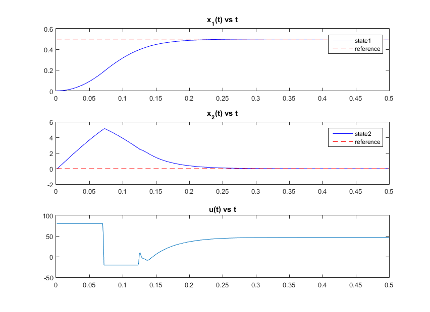
Results

In figure below, results for the above code are shown. x(1) and x(2) are states of system described in tutorial objectives. The red dashed lines represent the desired reference for each state. The u(t) represents solution of MPC controller.

Citation

If you use our code we kindly ask to cite the following paper:

Supplemental Information

This tutorial is a part of VSA project at ARMS Lab of Nazarbayev University

If you spot a typo in the tutorial or bug in the source code, please contact us via email:

• Bexultan Rakhim (bexultan.rakhim [at] nu.edu.kz )
• Olzhas Adiyatov (oadiyatov [at] nu.edu.kz )

or file an issue through GitHub.